In our November REALM meeting, we covered recent research under the theme of global ecohydrology. We were delighted to have two guest speakers, Dr Thanos Paschalis from the department of civil and environmental engineering, ICL and Dr Manon Sabot, a postdoctoral researcher at the University of New South Wales, currently at the University of Bristol as a visiting academic.

Here is a summary of the following talks:
- Giulia Mengoli: P-model performance in dry areas. Eco-evolutionary optimality theory applied to carbon, water, and energy cycle forecasting.
- David Sandoval: An appraisal of the development and testing of SPLASH v2.0: water and energy fluxes.
- Thanos Paschalis: On the uncertainty induced by pedotransfer functions in terrestrial biosphere modelling.
- Manon Sabot: Predicting resilience through the lens of competing adjustments to vegetation function. A case study in south-eastern Australia.
P-model performance in dry areas. Eco-evolutionary optimality theory applied to carbon, water, and energy cycle forecasting.
Giulia Mengoli
The latest version of the P-model has been implemented at a half-hourly timestep, and it is able to reproduce well the daily cycle of GPP in well-watered sites (Mengoli et al., 2022). However, in dry environments, the sub-daily P-model tends to overpredict GPP and it does not mimic the diurnal cycle of GPP either. So, at sub-daily timestep there are errors in the magnitude and in the shape of the GPP curve. The problem is that the current sub-daily version does not include the soil moisture limitation on GPP. In the P model GMD paper (2020) an empirical soil moisture stress function was presented and directly applied to downscale the GPP. Also land surface models make use of other soil moisture stress functions to reduce the tendency of the models to overestimate under water-stress conditions. However, we are not sure that by using an empirical soil moisture stress function we could be able to accurately mimic the diurnal cycle of GPP. But how to solve this?
Attempt 1: Process-based approach where the main logic was to control GPP via hydraulics rather than stomata. Could this process-based approach address the following research questions:
- Does the soil moisture act as a limiting factor for GPP?
- How low should the soil moisture be?
- Does the soil moisture change the stomatal sensitivity to VPD (Vapour Pressure Deficit)?
- Will this approach be enough to solve both problems (i.e., error in magnitude and shape)?
However, there were many problems with this process-based approach. There were issues with converting the soil water content from ECMWF to the matric potential, not knowing which soil types were in each site or how reliable the parameters were. It is possible, but this approach is not easy to implement.
Attempt 2: Empirical approach– the empirically derived factor (β(θ), ∈ [0, 1]∈0, 1), that captures the response of GPP to soil moisture stress requires estimation of plant-available soil water, expressed as a fraction of available water holding capacity and a measure of the local mean aridity, as the ratio between actual and potential evapotranspiration. Using the simulated soil moisture from the third-generation LSM at ECMWF (CTESSEL) the empirical soil moisture function was applied in the sub-daily P model.
The French evergreen broadleaf forest (FR-Pue) and several Australian sites have different vegetation and are affected in diverse ways by low soil moisture. Using the β(θ) application (the red line- the first layer of soil moisture from ECMWF, daily trends of GPP over different years), we were able to reduce the GPP from what we see in well-watered GPP (purple line).
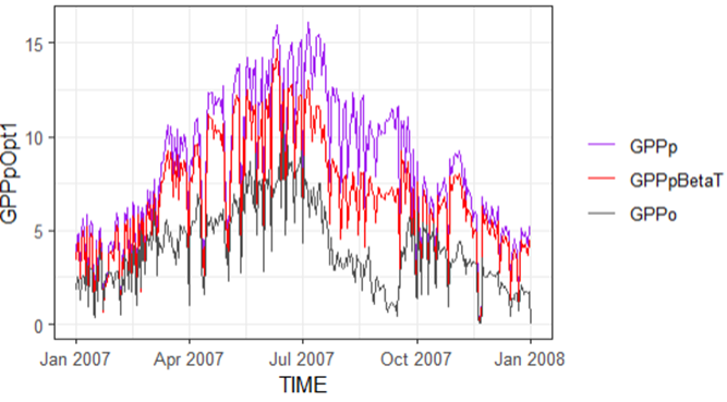
All the sites investigated (FR-Pue, AU-Stp, AU-Gin, AU- DaS) followed the same pattern as we can see in Figure 1 for FR-Pue in 2007-2008. The key point is that by using the empirical approach, we can reduce GPP but not enough to mimic what is observed, especially when the soil moisture is exceptionally low. Recalibration may be required.
Another aspect is that we need to factor in wilting point into our soil moisture stress function i.e., the input of the function needs to be θ as a fraction of available water holding capacity (the difference between the field capacity and wilting point). However, this needs the use of fixed parameters (i.e., wilting point and field capacity) that are soil-type specific, and not always reliable. Two ways of normalising this quantity led to different results.
- Normalising between 0 and 1 based on max and min of the θ series = GPPpBetaT
- Normalising subtracting wilting point and dividing by the difference = GPPpBetaTc
Some of the sites showed negative values if the latter normalising way was used, indicating soil moisture is lower than the wilting point, which is not possible.
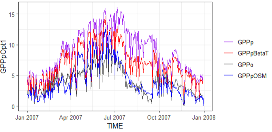
When we included in the results of GPP from the CTESSEL model (blue line, GPPpOSM), we can see that this more accurately follows the pattern observed (grey) than our models for this site (FR-Pue). But again, this pattern was not replicated at all sites.
The focus now is to improve this empirical function to obtain results that are closer to the observed, by investigating the β(θ) ratio and excluding the contribution of VPD because it does not appear to be a relationship between soil moisture and VPD.
An appraisal of the development and testing of SPLASH v2.0: Water and energy fluxes
Dr David Sandoval
SPLASH v2.0 (Simple process-led algorithms for simulations habitats) (SPLASH v2.0) builds on SPLASHv1.0 to allow robust calculations of water and energy fluxes in complex terrain. It is a simple, parsimonious model based on first principles, which does not require local calibration and uses minimum meteorological inputs (precipitation, air temperature and solar radiation). It works using analytical solutions for the integrals of the daily cycles and soil hydraulic transmissivity allowing the model to perform calculations at high spatial resolution without inflating the need for computational power. David gave an appraisal of the development and testing of SPLASH v2.0 and how it compares to other predictive modelling tools on the following aspects of ecohydrology:
- Net radiation
- Evapotranspiration
- Snowpack
- Surface runoff and lateral flow
- Soil moisture
- Condensation
- Soil water storage and conductivity
To read more about the results of this appraisal, check out the follow blog article by David:
On the uncertainty induced by pedotransfer functions in terrestrial biosphere modelling.
Dr Thanos Paschalis, guest speaker
The movement of water through soil is a key part of the water and carbon cycle, but it is difficult to observe. Due to this lack of in-situ data, many ecosystems and hydrological modelling tools parametrize soil hydraulic properties using widely available information on soil texture. Several empirical models, or pedotransfer functions (PTFs), are currently available but their predictions are commonly vastly different. The aim of our recent study (in Water Resources Research) was to quantify how uncertainties in soil hydraulic properties can propagate to hydrological and ecosystem dynamics.
When we use pedotransfer functions (PTFs) in ecosystem modelling, we introduce uncertainty into the model because the soil’s hydraulic properties such as the hydraulic conductivity and its water retention curve are uncertain quantities. In this study, we wanted to quantify this uncertainty and how this propagated into the water and carbon cycles. Additionally, we wanted to understand the impacts of climate, soil type and topography on these uncertainties.
Using the T&C terrestrial ecosystem model, we ran 3 simulations using 7 PTFs that come from 2 models (Brooks-Corey Model and the Mualem-van Genuchten model).
- Sites x PTFs: one-dimensional simulation using local meteorology, soil texture and plant traits. Using 70 sites and 7 PFTs.
- Sites x PTFs x soil types: one-dimensional simulation using 70 sites, 7 PFTs, but prescribing soil types from 12 soil classes (sandy to heavy clay).
- Sites x PTFs x soil types x topography: three-dimensional simulation using a small catchment to perform No.2 simulations but including topography.
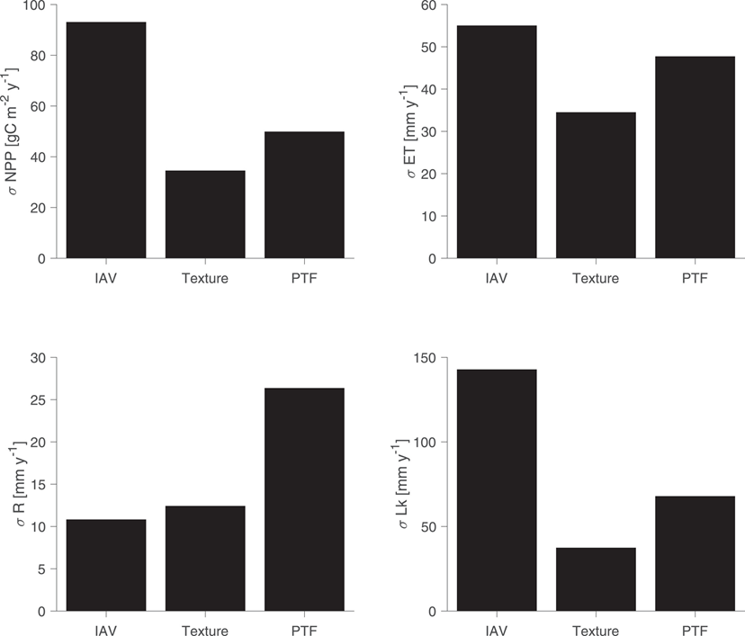
Our results showed that the choice of PTF alone introduced huge variations (up to 2-fold) in NPP. The uncertainties were largest for hydrological fluxes, especially runoff and groundwater recharge. We also found that uncertainties between PTFs are comparable to uncertainties in the soil texture.
When we considered the background climate, i.e., how wet or dry a site was, the choice of PTF introduced an uncertainty of 10% of the actual rainfall that is received at the driest sites, which is very considerable. This uncertainty gets smaller as we move into wetter sites. For example, if you have a very rainy year in a dry area, you will get more productivity in the dry site, this is less pronounced in an already saturated site.
Topography had a significant impact and where you were in the catchment, i.e., how close you are to the river network and features such as valleys and mountains. It could either amplify or dampen the uncertainties by altering plant water stress. Therefore, we should consider topography when we run global-scale simulations.
You can read the full paper here:
Paschalis, A., Bonetti, S., Guo, Y. and Fatichi, S. 2022. On the uncertainty induced by pedotransfer functions in terrestrial biosphere modelling. Water Resources Research, 58(9), https://doi.org/10.1029/2021WR031871.
Predicting resilience through the lens of competing adjustments to vegetation function. A case study in south-eastern Australia.
Dr Manon Sabot, guest speaker
Understanding how ecosystems respond to drought is a pressing challenge. Whilst there has been work on incorporating eco-evolutionary optimality (EEO) theories into land-surface models (LSMs), so far, it has not been attempted to incorporate multiple or competing theories into modelling. In our recent paper in Plant, Cell, and Environment, we tried to infer new things about ecosystem resilience using different optimisation approaches. We coupled EEO approaches that optimize
- canopy gas exchange – assumed to be a trade-off between carbon gains (photosynthetic function) and hydraulic costs (hydraulic function) to the vegetation
- leaf nitrogen allocation (Nopt) – how to invest leaf nitrogen to maximize photosynthetic function
- hydraulic legacies (Hleg) – to account for hydraulic impairment during times of drought
We tested our model at EucFACE, a Free-Air Carbon Dioxide Enrichment experiment in Australia, using observations from 6 plots of native Eucalyptus woodland. This site is both water- and nutrient-limited and experienced repeated droughts and heatwaves between 2013 and 2020. We had 3 plots at ambient CO2 and 3 at elevated CO2.
We established that the model configurations were affected in a predictive and interpretable manner along axes of variation in soil moisture, LAI (Leaf Area Index) and CO2. We also found that the model responses best matched the observations we had from the sites if we optimized Vcmax and Jmax more frequently. Our best model configuration accounted for Nopt every 7th day and Hleg every 30th day, whilst canopy gas exchange was optimized every half hour by default (canopy gas exchange is resolved on relatively short timescales in LSMs).
With this model configuration, we wanted to assess our model predictions of adjustments to function, e.g., to see how Vcmax and Jmax vary with ecosystem fluxes and changes to the environmental conditions. We also wanted to explore the relationships between drought-driven foliage dynamics and plant hydraulic function.
Predicted adjustments to function (best model configuration)
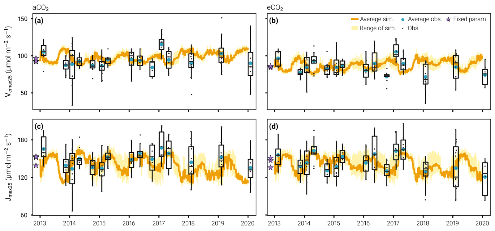
Figure 1. The timeseries of theVcmax25 (a and b) and Jmax25 (c and d) predicted by the best model configuration (Hleg= 30 days, Nopt= 7 days) and compared with field observations at the ambient CO2 (a and c) and elevated CO2 (b and d) plots. Orange lines show the average simulations across plots and yellow shadings the range of simulations. Box and whisker plots summarize the observed distributions of Vcmax25 and Jmax25 (line, median; box, interquartile range; whiskers, quartiles ± 1.5 times the interquartile ranges).
What we can see from Figure 1 is that the model has captured the seasonal shifts in Jmax well. In late spring and early summer (i.e., November/December), we have a low Jmax at EucFACE and then it increases to peak in winter (July/August) before it decreases again, which effectively follows the hydrological year in Australia. However, in late spring and early summer, the Vcmax predictions are too high: there are very few leaves, and we do not know whether the optimality criterion does not work when the leaf area index (LAI) is very low (~0.5 m2 m-2), or whether the scattering of radiation throughout the canopy does not work well in these conditions, or both. Overall, though, the gross primary productivity (i.e., carbon uptake) is limited by Jmax more than by Vcmax at this site, even when the LAI is low, so there is no strong constrain on Vcmax in our model.
Understanding the lack of simulated hydraulic legacy: foliage response to drought
When we explored the responses to ecosystem fluxes, we were surprised to see that hydraulic legacy effects on transpiration fluxes were small and short-lived (2 months). We asked ourselves, what would happen to the vegetation if there was only one LAI phenology that varied during the year but was constant at the same time each year?
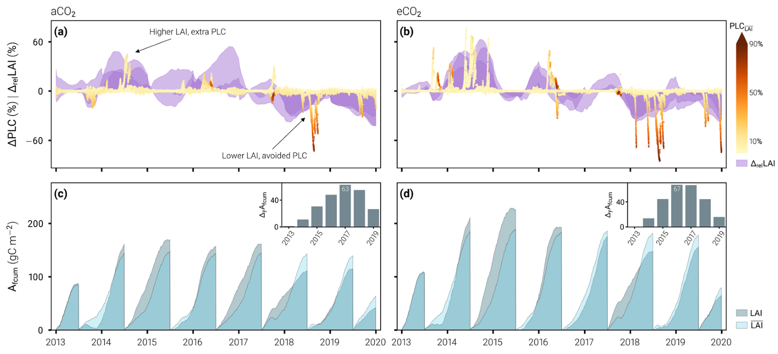
Figure 2. The relative costs and benefits associated with deviations in leaf area index (LAI) from the average phenology (LAI) at the aCO2 (a and c) and eCO2 (b and d) plots, as simulated by the best model configuration. (a) and (b) shows the time-series of the percentage point changes in canopy percentage loss of hydraulic conductivity (ΔPLC) associated with percentage changes in LAI relative to the average phenology of each plot (ΔrelLAI). (c) and (d) show the cumulative portion of assimilated carbon that is allocated to leaf growth (Afcum) over the hydrological year (July 1st to June 31st), depending on the LAI prescribed in the model simulations. Inset plots show the cumulated differences in Afcum at the end of each hydrological year (ΔyAfcum).
In Figure 2 we ran our best model configuration using a fixed average LAI phenology, and we got vastly different results compared to when we used the observed LAI phenology that varies from year to year. In the top panels, positive purple shading means that the observed LAI was higher than you would expect for “an average year,” and vice versa. The yellow to dark red scatter shows the associated difference in canopy hydraulic status, i.e., the percentage loss of hydraulic conductivity (PLC) difference incurred from adjustments to LAI in any given year. In wet years (e.g., 2013-2015), the trees are growing leaves and risking extra losses of hydraulic conductivity (extra PLC) in the canopy, but there is no baseline hydraulic stress (the scatter is a pale yellow) and therefore recovery from this extra PLC should be quick. By contrast, in dry years (2017 onwards), the trees are dropping leaves and thus avoiding large extra hydraulic conductivity losses, which would have occurred in addition to considerable hydraulic stress due to drought (the scatter is a dark red). The bottom panels show higher increasing cumulative carbon storage for the model forced with observed LAI (dark blue) compared to the average LAI phenology (pale blue), until either 2016 (eCO2 rings) or 2017 (aCO2). After those years, the LAI declined greatly, reducing carbon uptake and storage. Taking the top and bottom panels together, we can say that because the trees grew leaves in the wet years and were able to assimilate a lot of carbon, they could then afford to lower their LAI during drought and avoid considerable damage to their hydraulic function.
This analysis suggests that leaf shedding and/or suppressed foliage growth is a strategy to mitigate drought risk. Accounting for foliage responses to water availability has the potential to improve model predictions of ecosystem resilience.
You can read the full paper here:
Sabot, MEB, De Kauwe MG, Pitman AJ, Ellsworth DS, Medlyn BE, Caldararu S, Zaehle S, Crous KY, Gimeno TE, Wujeska-Klause A, Mu M, Yang J. 2022. Predicting resilience through the lens of competing adjustments to vegetation function. Plant Cell Environ, 45(9):2744-2761. Doi: 10.1111/pce.14376.
